Table of Contents
1. Summary, Aknowledgment and links
1.1. Useful links
This page contains notes and links on Variational inference or Variational Bayes. The content is mainly inspired by different readings:
- Christopher Bishop's book (see chapter 9 and 10 of Pattern Recognition and Machine Learning)
afor "statisticians"
- The tutorial at NIPS 2016 by Blei et al.; it includes recent stochastic approaches to Variational Inference
- The talk of Kay H. Brodersen; it starts with Laplace approximation and covers density estimation, regression and clustering.
1.2. Introduction
Consider a probabilistic model in which we denote all the observed variables by \(\X\) and all the hidden variables by \(\Z\). In general, the probabilistic model is designed by a generative story which implies a definition of the joint probability \(P(\X, \Z|\pa)\) or \(P(\X, \Z,\pa)\) in the real bayesian view.
If we consider the joint distribution \(P(\X, \Z|\pa)\), it is defined by a set of parameters denoted \(\pa\). The goal is to maximize the likelihood function \(P(\X|\pa)\) to learn the parameters \(\pa\). However, this maximization problem is intractable in most of the case.
If we consider \(P(\X, \Z,\pa)\), there are different levels of bayesian inference:
- infer \(P(\pa|\X)\) which also implies a summation over \(\Z\)
- infer \(P(\X)\) for prediction purpose
- infer \(P(\Z|\X,\pa)\), the posterior distribution of the latent variable to better analyse new data.
In all cases, the inference is untractable because we need to estimate \(P(\X|\pa)\) or even marginalize parameters. This requires approximate inference approach, such as MCMC or Variational one.
1.3. Remarks on notation and random variables
It is difficult to clearly define notation to handle all cases. For instance, let us consider a Gaussian mixture model. It can be used for density estimation or data clustering. Observed variables \(\X\) are random vectors, each belonging to a cluster. The affectations of each example to a cluster (or a gaussian) is encoded by \(\Z\) the set of latent variables. The model is defined by its set of parameters \(\pa\).
In Bayesian perspective, the parameters are also considered as random variables and therefore \(\pa\) can be included in \(\Z\). In this case, parameters are treated as random variables, just like affectations. However, there is an important difference between \(\pa\) and \(\Z\):
- \(\Z\) are local random variables, there is one affectation by training example;
- \(\pa\) are global random variables, they are shared across the training data.
This can represent a an issue for scalability. For each training example, you have to store the distribution over its affectation or its associated random variable. For large corpus, this is not convenient. More recent approaches rely on stochastic variants of Variational Inference as an efficient work-around.
To summarize this distinction:
- In the MLE, we consider \(P(\X, \Z|\pa)\) to estimate a value of \(\pa\). We can also estimate \(P(\Z|\X,\pa)\).
- In the Bayesian case, we consider \(P(\X, \Z, \pa)\) to estimate a value of the posterior distributions over \(\pa\) and \(\Z\).
1.4. Expectation of a random variable
Before to read these notes, it is better to be familiar with expectation. Given a random variable \(X\), we define its expectation under the distribution \(p\)
\begin{align} E_{X \sim p}[X] &= \sum_{x} p(X=x) x \\ &\int_x p(x) x dx \end{align}The first line is for discrete RV while the second one is for continuous RV. In this last case, \(p(x)\) denotes the probability density function. If \(X\) is a categorical RV, note it can be meaning less as it is, while for continuous RV it can be interpreted as the mean value.
A quantity of interest is the expected value of a function of the RV. For instance, the variance of a continuous RV can be expressed as \(E[(X-E[X])^2]\). In information theory, it is meaningfull to define the expected value of the information quantity as the entropy of the RV \(X\): \[ H(X)=-\sum_x p(X=x)log(p(X=x)) = E_p[-log(p(X))] \]
Now assume two distributions on the same RV, \(q\) and \(p\), we can measure the Kullback-Leibler divergence between these two distributions as :
\[ \dkl(p||q)=\sum_x p(X=x)log(p(X=x)/q(X=x)) = E_p[log(p(X)/q(X))] \]
This divergence is not symmetric, \(\dkl(p||q) \neq \dkl(q||p)\), and is \(\geq 0\). The equality stands when \(p\) and \(q\) are the same distribution over \(X\).
If we denote \(p^*\) the true distribution of \(X\) and if we parametrize a distribution over \(X\) with \(\pa\), we can search \(\pa\) to minimize the following divergence:
\begin{align*} \dkl(p^*||p_{\pa}) &= \sum_x (p^*(X=x)log p^*(X=x)-p^*(x) log(p_{\pa}(X=x)))\\ &= \sum_x p^*(X=x)log p^*(X=x)- \sum_x p^*(x) log(p_{\pa}(X=x))\\ &= Cste - \sum_x p^*(x) log(p_{\pa}(X=x))\\ &= Cste - E_{X\sim p^*} [log p_{\pa}(X=x)] \end{align*}Therefore minimizing this theoritical KL divergence is equivalent to maximizing in practice the log-likelihood wrt \(\pa\).
2. Variational Bayes: Bayesian "approximate (or not)" inference
This likelihood can be expressed in two ways: \[P(\X|\pa)= \sum_{\Z} P(\X,\Z|\pa)= \frac{P(\X,\Z|\pa)}{P(\Z|\X,\pa)}\].
The "untractability" comes from marginalization: in the first case, sum over \(\Z\); while in the second case, the same issue is hidden in the latent posterior distribution \(P(\Z|\X,\pa)\). Let us consider the second one in its log formulation:
\(\log(P(\X|\pa))= \log(\frac{P(\X,\Z|\pa)}{P(\Z|\X,\pa)})\)
2.1. Variational derivation
Let introduce a distribution \(q(\Z)\) defined over the latent variables. This probability function is an approximate of the true posterior \(P(\Z|\X,\pa)\). The goal is to find the distribution \(q\) that best approximates the posterior distribution and then to use it as a proxy for Bayesian inference.
To introduce \(q\), we can multliply both parts of the previous equation with \(q\), and sum over \(\Z\):
\(\sum_{\Z} q(\Z) \log(P(\X|\pa))= \sum_{\Z}\log(\frac{P(\X,\Z|\pa)}{P(\Z|\X,\pa)})q(\Z)\)
The right hand side is just \(P(\X|\pa)\) and remains unchanged. The second trick is to introduce \(q(\Z)\) in the fraction:
\(\log(P(\X|\pa))= \sum_{\Z}q(\Z) \log(\frac{P(\X,\Z|\pa)q(\Z)}{P(\Z|\X,\pa)q(\Z)})\)
Then reformulate it a little bit:
\(\log(P(\X|\pa))= \sum_{\Z}q(\Z) \log(\frac{P(\X,\Z|\pa)}{q(\Z)}) + \sum_{\Z}q(\Z) \log(\frac {q(\Z)}{P(\Z|\X,\pa)})\)
Two terms appear. The second one is the Kullback-Leibler divergence between \(q(\Z)\) and \(P(\Z|\X,\pa)\): \[ \dkl(q(\Z)||P(\Z|\X,\pa)) = \sum_{\Z} q(\Z) \log(\frac{q(\Z)}{P(\Z|\X)}). \] And the first term is for the moment denoted by \(\lb\).
2.2. Evidence Lower Bound, or the ELBO
We then obtain the following relation:
\begin{align} \log(P(\X|\pa)) &= \lb + \dkl(q(\Z)||P(\Z|\X,\pa))\\ \lb &= \sum_{\Z}q(\Z) \log(\frac{P(\X,\Z|\pa)}{q(\Z)}) \\ &= E_{q}[ \log(\frac{P(\X,\Z|\pa)}{q(\Z)}) ] \\ &= E_{q}[ \log(P(\X|\Z, \pa) ] - \dkl(q(\Z)| P(\Z))\\ &= E_{q}[ \log(P(\X, \Z | \pa) ] + H(q) \end{align}Recall that the Kullback-Leibler divergence satisfies \(\dkl(q|p)\ge 0\), with equality if, and only if \(q(\Z) = p(\Z|\X,\pa)\). Therefore \(P(\X|\pa) \ge \lb\) which means that \(\lb\) is a lower bound of \(P(\X|\pa)\) we want to maximize. \(\lb\) is therefore named the Evidence Lower Bound or \(\elbo\).
This formulation does not solve the tractability issue since in the \(\dkl\) term we still have a dependance between \(P(\Z|X,\pa)\) and \(P(\X|\pa)\), i.e :
\(P(\Z|X,\pa) = \frac{P(\X,\Z|\pa)}{P(\X|\pa)}\).
So both \(P(\Z|X,\pa)\) and \(P(\X|\pa)\) are untractable. The probabilistic model specifies the joint distribution \(P(\X, \Z)\), and the goal is to find an approximation for the posterior distribution \(P(\Z|\X,\pa)\) as well as for the model evidence \(P(X|\pa)\).
To quote Christopher Bishop (see chapter ten of Pattern Recognition and Machine Learning):
Although there is nothing intrinsically approximate about variational methods, they do naturally lend themselves to finding approximate solutions. This is done by restricting the range of functions over which the optimization is performed, for instance by considering only quadratic functions or by considering functions composed of a linear combination of fixed basis functions in which only the coefficients of the linear combination can vary. In the case of applications to probabilistic inference, the restriction may for example take the form of factorization assumptions
2.3. Approximate inference
To solve the tractability issue, there are two common approaches:
- The E.M algorithm that fix the parameters during the E step and then compute when it's possible \(P(\Z|\X;\pa)\) to then optimize the \(\elbo\).
- Otherwise we can directly optimize the \(\elbo\) term. This can be done with some further assumptions on \(q\) like mean-fields.
3. A special case: EM
The EM algorithm aims at estimating the parameters \(\pa\) of a generative model that relies on latent variables \(\Z\) to explain the observed data \(\X\). In the example of mixture of gaussians, \(\Z\) represents the affectation of each observation to a gaussian. If \(\Z\) could be observed, it becomes therefore a simple and easy to solve classification problem. We can call \((\X, \Z)\) the complete data set, while \((\X)\) is the incomplete one. In other words, \(P(\X,\Z|\pa)\) is easy to optimize, while \(P(\X|\pa)\) is untractable (the log-sum).
However, in practice \(\Z\) is unknown, but for a given set of parameters we can compute \(P(\Z|\X,\pa)\) and also the expected value of \(\Z|\X,\pa\). This is the E(xpectation) step. In a second step, the classification task can be carried out: maximizing \(\pa\) knowing \(\Z\) (or the expected value). This is the M(aximization) step.
As written in the review of (Blei et al.), EM optimize the expected complete log-likelihood and this is the first term of the ELBO. The goal of the algorithm is to find maximum likelihood estimates for parameters in models with latent variables. Parameters are in this case not considered as random hence latent variables. Unlike Variational Inference, EM assumes that the posterior distribution \(P(\Z|\X,\pa)\) is computable. Unlike EM, variational inference does not estimate fixed model parameters but it is often used in a Bayesian setting where classical parameters are treated as latent variables.
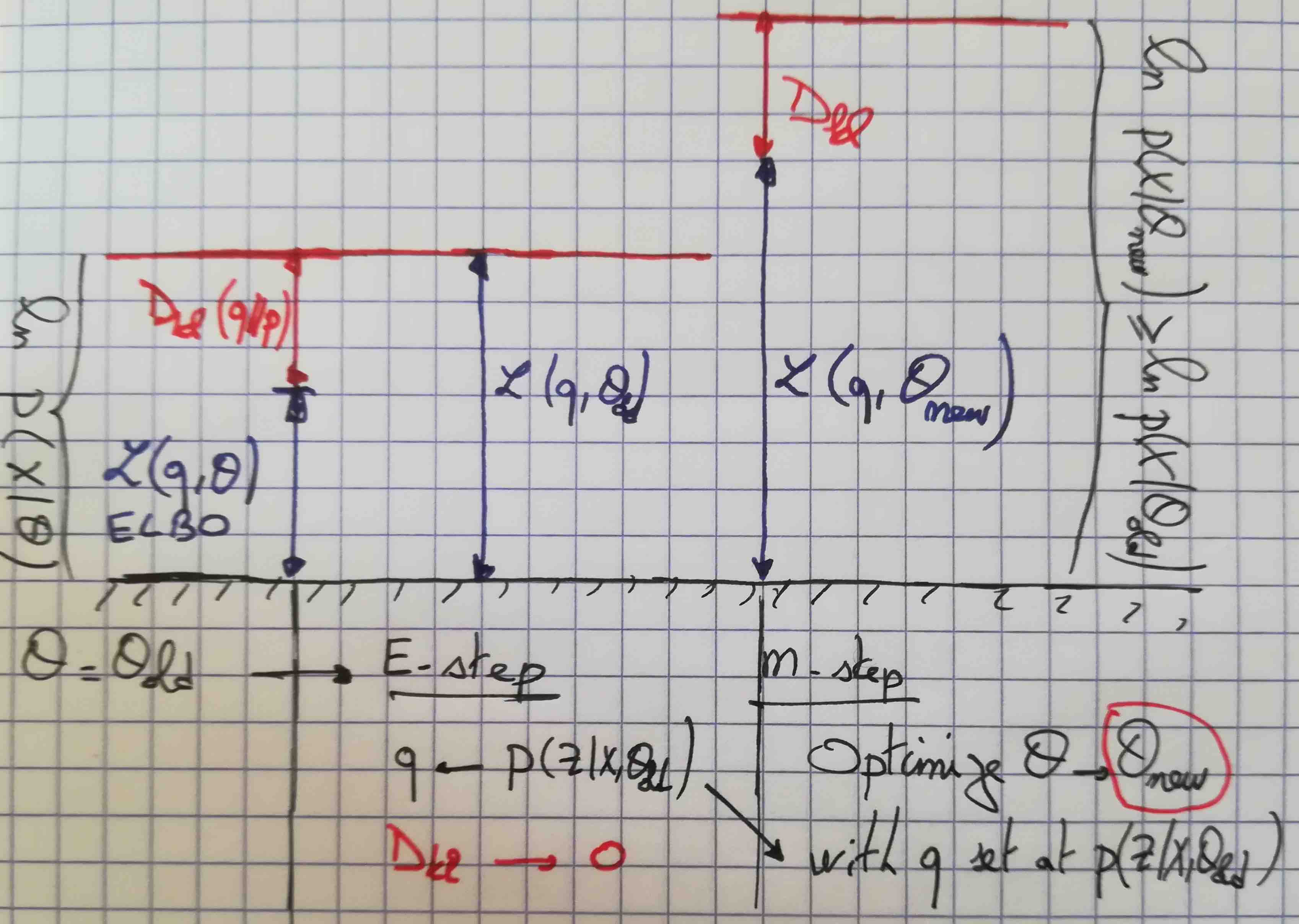
Now we can go back to the lower bound to explain the EM algorithm. This is a two-stage iterative optimization technique for finding maximum likelihood solutions.
3.1. E step
Suppose that the current value of the parameter vector is \(\paold\). In the E step, the lower bound \(\lb\) is maximized with respect to \(q(\Z)\) while holding \(\pa\) fixed to \(\paold\). If you remember that:
- \(P(\X,\Z|\paold)=P(\Z|\X,\paold)P(\X|\paold)\),
- so the solution is when \(q(\Z) = P(\Z|\X,\paold)\).
- Therefore, the Kullback-Leibler divergence vanishes.
Since the KL divergence is zero, we have \(\lb=P(\X|\paold)\). In fact, the E-step consists in computing the posterior distribution over \(\Z\) with the parameters fixed at \(\paold\). Then you just set theoritically \(q(\Z) = P(\Z|\X,\paold)\).
3.2. M step
The distribution \(q(Z)\) is now fixed and the lower bound \(\lb\) is now maximized with respect to \(\pa\). The maximization process yields a new value for the parameters \(\panew\) and increases the lower bound (except if we are already at the maximum). Note that \(q(Z)=P(\Z|\X,\paold)\) acts as a constant in the maximization process:
\begin{align} \lb &= \sum_{\Z} P(\Z|\X,\paold) \log(\frac{P(\X,\Z|\pa)}{P(\Z|\X,\paold)}) \\ &= \sum_{\Z} P(\Z|\X,\paold) \log(P(\X,\Z|\pa)) - \sum_{\Z} P(\Z|\X,\paold) \log(P(\Z|\X,\paold)) \end{align}The second term is a positive constant, since it depends only on \(\paold\). This is the entropy of the posterior distribution \(H(P(\Z|\X,\paold))\). The first we want to maximize is the expectation under the posterior \(P(\Z|\X,\paold)\) of the log-likelihood of complete data. This means in practice, that we optimize a classifier of \(\X\) into \(\Z\), with the supervision of \(P(\Z|\X,\paold)\) that provides the pseudo-affectation.
Since the distribution \(q\) is fixed to \(P(\Z|\X,\paold)\), \(q(Z) \neq P(\Z|\X,\panew)\) and now the KL divergence term is nonzero. The increase in the log likelihood function is therefore greater than the increase in the lower bound.
3.3. A summary of EM
You can see the EM algorithm as pushing two functions.
- With fixed parameters (\(\paold\)), push \(\lb\) to stick \(P(\X|\paold)\) by setting \(q(Z)=P(\Z|\X,\paold)\)
- Then recompute the parameters to get \(\panew\) with a fixed \(q(\Z)=P(\Z|\X,\paold)\). The criterion is to maximize \(\lb\) w.r.t \(\pa\). In fact you are moving in the parameter space in order to push \(\lb\), but by doing this you also push the likelihood even further: \(P(\X|\panew) \ge \lb\) because \(P(\Z|\X,\pa)\) has changed to \(P(\Z|\X,\panew)\) while \(q(\Z)\) has not.
For graphical illustration, you can look at the book of Christopher Bishop called Pattern Recognition and Machine Learning. You can also read the great paper of Radford Neal and Geoffrey Hinton on the link between Variational Bayes and EM.
Note that for implementation, \(q(\Z)\) does not really exist or is not a quantity of interest. It acts more like a temporary variable to perform this two steps game.
4. The problem of approximate inference in general
In this part, there is no mention of hyperparameters or even parameters. Let say that the latent variables represent all unknown quantities of interest.
A generative model defines a joint density of latent variables \(\Z\) and observations \(\X\), \[p(\Z, \X) = p(Z)p(\X | \Z),\] with a generative scenario: draw the latent variables from a prior density \(p(\Z)\) and then relates them to the observations through the likelihood \(p(\X|\Z)\). Inference in a Bayesian model amounts to conditioning on data and computing the posterior \(p(\Z | \X)\). In fact, the latent variables \(\Z\) help govern the distribution of the data.
To estimate \(p(\Z|\X)\), the Bayes formula tells us:
\[p(\Z|\X) = \frac{p(\X,\Z)}{p(\X)}\]
This is not of a great help since the denominator is the evidence and is also untractable: the summation over all the possible values of \(\Z\).
4.1. The evidence lower bound (ELBO).
Given a family of distribution, we are looking for one its member \(q(\Z)\) that best approximates the conditional distribution \(p(Z|X)\). The criterion is the Kullback-Leibler divergence :
\(q^*(\Z) = argmin_{q} \dkl(q(\Z)||p(\Z|\X))\)
This objective is not tractable since its relies on \(p(\Z|\X)\) and hence on \(p(\X)\) :
\begin{align} \dkl(q(\Z)||p(\Z|\X)) &= E_{q}[\log q(\Z)] - E_{q}[\log p(\Z|\X)]\\ &= E_{q}[\log q(\Z)] - E_{q}[\log p(\X,\Z)] + E_{q}[\log p(\X)]\\ &= E_{q}[\log q(\Z)] - E_{q}[\log p(\X,Z)] + \log p(\X)\\ \end{align}This shows the dependence of the objective on the data evidence, but also that \[\dkl(q(\Z)||p(\Z|\X)) \ge E_{q}[\log q(\Z)] - E_{q}[\log p(\X,\Z)].\] Minimizing the second term is equivalent to minimize the KL divergence objective. The term \(\log p(\X)\) is independent of \(q(\Z)\) and thus a negative constant.
The quantity \(E_{q}[\log p(\X,\Z)]- E_{q}[\log q(\Z)]\) is called the evidence lower bound (ELBO). The term ELBO comes from the fact that if you reorganise the equation, you get:
\begin{align} \log p(\X) &= \dkl(q(\Z)||p(\Z|\X))+ E_{q}[\log p(\X,\Z)]- E_{q}[\log q(\Z)] \\ &= \dkl(q(\Z)||p(\Z|\X)) + \elbo(q) \\ &\ge \elbo(q) \end{align}Therefore maximizing the elbo term implies both to find the best approximate \(q(\Z)\) within a family of distribution of \(p(\Z|\X)\) and also to maximize a lower bound of \(p(\X)\).
For further insight, the elbo can be rewritten as:
\begin{align} \elbo(q)&= E_{q}[\log p(\Z)] + E_q [\log p(\X|\Z)]- E_q [\log q(\Z)]\\ &= E_q [\log p(\X|\Z)] - \dkl(q(\Z)||p(\Z)) \end{align}The first term is an expected log likelihood under the \(q\) distribution and the second is the divergence between the variational density and the prior. Therefore maximizing \(\elbo(q)\) resorts to maximizing the expected log likelihood under the \(q\) distribution, while keeping \(q\) as close as possible to the prior \(p(\Z)\).
Second derivation of the ELBO: In a lot of papers and books on variational inference, the elbo is derived through Jensen's inequality. See the Jordan's paper in 1999 for instance.
\begin{align} \log p(\X) &= \log \sum_{\Z} p(\X,\Z) = \log \sum_{\Z} \Big[ p(\X,\Z)\frac{q(\Z)}{q(\Z)}\Big] \\ &= \log E_q \Big[\frac{p(\X,\Z)}{q(\Z)}\Big] \\ &\geq E_q \Big[ \log \frac{p(\X,\Z)}{q(\Z)}\Big] \\ &= E_q \Big[ \log p(\X,\Z)\Big] + H(\Z) \end{align}See the swap between the \(\log\) function and the expectation: this is the application of the Jensen's inequality.
Remark: The Jensen equality states that for a convex function, while the \(\log\) function is concave ! But some books and papers, "convex" is used for both convex and concave, adding an adjective "upward" or "downward" (can be confusing).
4.2. ELBO : some comments
Variational inference aims at maximizing the ELBO. This means that we indirectly optimize two terms:
- maximizing \(p(\X)\), the data evidence, while
- minimizing the divergence \(\dkl(q(\Z)||p(\Z|\X))\).
The elbo term can be written as:
\begin{align} \lb &= E_{q}[\log p(\X,\Z|\pa)]- E_{q}[\log q(\Z)] . \end{align}Maximizing the ELBO, means thus to jointly maximize \(E_{q}[\log p(\X,\Z|\pa)]\) and the entropy of the distribution \(q\). With the first term, \(q\) should put probability mass on \(\Z\) to explain the data. The second term favours otherwise uniform distribution.
However we can further decompose the joint distribution:
\begin{align} \lb &= E_{q}[\log p(\X|,\Z,\pa) p(\Z|\pa)]- E_{q}[\log q(\Z)] \\ &= E_{q}[\log p(\X|,\Z,\pa)] + E_{q}[p(\Z|\pa)-\log q(\Z)] \\ &= E_{q}[\log p(\X|,\Z,\pa)] - \dkl( q(\Z)||p(\Z|\pa) ). \end{align}With the first term, \(q\) will tend to place probability mass on configurations of the latent variables that explain the observed data. For example, if you compute the first term with Monte-Carlo methods, the density \(q\) should propose values of \(\Z\), for which \(p(\X|\Z,\pa)\) is high. The second term is the negative KL divergence between the \(q\) and the prior distribution. It favors distributions close to the prior. Therefore the second term can be interpreted as a régularization term on \(q\).
4.3. TODO Example of variational inference
As in the Bishop's book or the review of Blei et al., the Bayesian mixture of gaussians could be a good example to write.
5. Variational inference or MCMC
Here is quoted, what you can read in this review from Blei et al., comparing variational inference and MCMC:
When should a statistician use MCMC and when should she use variational inference? We will offer some guidance. MCMC methods tend to be more computationally intensive than variational inference but they also provide guarantees of producing (asymptotically) exact samples from the target density (Robert and Casella, 2004). Variational inference does not enjoy such guarantees it can only find a density close to the target but tends to be faster than MCMC. Because it rests on optimization, variational inference easily takes advantage of methods like stochastic opti- mization (Robbins and Monro, 1951; Kushner and Yin, 1997) and distributed optimization (though some MCMC methods can also exploit these innovations (Welling and Teh, 2011; Ahmed et al., 2012)).
Thus, variational inference is suited to large data sets and scenarios where we want to quickly explore many models; MCMC is suited to smaller data sets and scenarios where we happily pay a heavier computational cost for more precise samples. For example, we might use MCMC in a setting where we spent 20 years collecting a small but expensive data set, where we are confident that our model is appropriate, and where we require precise inferences. We might use variational inference when fitting a probabilistic model of text to one billion text documents and where the inferences will be used to serve search results to a large population of users. In this scenario, we can use distributed computation and stochastic optimization to scale and speed up inference, and we can easily explore many different models of the data.
Data set size is not the only consideration. Another factor is the geometry of the posterior distribution. For example, the posterior of a mixture model admits multiple modes, each corresponding label permutations of the components. Gibbs sampling, if the model permits, is a powerful approach to sampling from such target distributions; it quickly focuses on one of the modes. For mixture models where Gibbs sampling is not an option, variational inference may perform better than a more general MCMC technique (e.g., Hamiltonian Monte Carlo), even for small datasets (Kucukelbir et al., 2015). Exploring the interplay between model complexity and inference (and between variational inference and MCMC) is an exciting avenue for future research (see Section 5.4). (…)